Interpretation of an Auto SARIMAX model output in R

The model we run is this

library(forecast)
library(ggplot2)

# Create sample data
set.seed(123)
n <- 120
time <- 1:n

# Main time series with trend + seasonality
y <- 50 + 0.3*time + 10*sin(2*pi*time/12) + rnorm(n, 0, 5)

# External variable (e.g., marketing spend)
x1 <- 20 + 0.1*time + rnorm(n, 0, 3)

# Convert to time series object
y_ts <- ts(y, frequency = 12)
x1_ts <- ts(x1, frequency = 12)

# Let R find optimal parameters
sarimax_model <- auto.arima(y_ts,
                            seasonal = TRUE,
                            stepwise = TRUE,
                            approximation = TRUE,
                            xreg = x1_ts)
summary(sarimax_model)

Now the output we get is

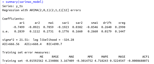
Interpretation

Here’s a comprehensive interpretation of our SARIMAX model output:

Model Structure

SARIMAX(2,0,1)(2,1,1)[12] with external regressor

• Non-seasonal part: AR(2) + MA(1)
• Seasonal part: Seasonal AR(2) + Seasonal MA(1) with seasonal differencing (D=1)
• Seasonality: 12 months (monthly data)
• External regressor: One predictor variable (xreg)

Coefficients Interpretation

Non-seasonal Components:

• AR(1) = -0.75: Strong negative autoregressive effect - high values tend to be followed by low values
• AR(2) = -0.09: Weak negative second-order autoregressive effect
• MA(1) = 0.79: Strong moving average effect - shocks persist for one period

Seasonal Components (12-month cycle):

• SAR(1) = -0.19: Moderate negative seasonal autoregressive effect
• SAR(2) = 0.04: Very weak positive seasonal effect
• SMA(1) = -0.85: Strong negative seasonal moving average - seasonal shocks reverse quickly

External Effects:

• Drift = 0.26: Positive trend component (0.26 units increase per period)
• xreg = 0.30: External variable has positive effect - 1 unit increase in xreg predicts 0.30 unit increase in y

Model Quality Assessment

Statistical Significance:

• Significant coefficients: AR(1), MA(1), SMA(1), Drift (coefficient > 2× standard error)
• Borderline: xreg (2.07× SE), SAR(1) (1.08× SE)
• Insignificant: AR(2), SAR(2) (coefficient < SE)

Model Fit Statistics:

• AIC = 666.56, BIC = 690.7: Good for model comparison (lower is better)
• Log-likelihood = -324.28: Baseline for model comparison
• σ² = 21.51: Error variance

Forecast Accuracy:

• RMSE = 4.23: Average forecast error magnitude
• MAE = 3.17: Average absolute error
• MAPE = 4.72%: Excellent accuracy (error <5% of actual values)
• MASE = 0.52: Model performs 48% better than naive forecast

Key Insights & Recommendations

Strengths:

1. Excellent predictive accuracy (MAPE <5%)
2. Strong seasonal patterns captured effectively
3. Good model fit with reasonable complexity
4. External variable adds value to predictions

Concerns:

1. Over-parameterization: AR(2) and SAR(2) appear unnecessary
2. Some coefficients borderline significant

Suggested Improvement:

# Try simplified model
better_model <- Arima(y_ts, order = c(1,0,1), seasonal = c(1,1,1), xreg = xreg)

Business Interpretation:

• The time series shows strong seasonal patterns with 12-month cycles
• There’s a positive underlying trend (0.26 units/period)
• The external variable has moderate predictive power
• Model provides highly accurate forecasts with ~4.7% average error

This is generally a good quality model that should provide reliable forecasts for business planning.