When Can the Binomial Distribution Be Approximated by the Poisson?
The binomial distribution B(n, p) is close to a Poisson(np) when n is large and p is small. We state the rule of thumb, work two examples, and check the approximation in R with ggplot2.
R
Statistics
Probability
Author
Abdullah Al Mahmud
Published
November 3, 2026
Working with binomial probabilities.
A binomial distribution \(B(n, p)\) can be approximated reliably by a Poisson distribution \(P(\lambda)\) when the number of trials \(n\) is large and the probability of success \(p\) is small. In other words, the approximation suits rare events counted over many trials. Let’s see the rule, two worked examples, and a picture of how good the fit is.
Why It Works
The binomial probability of \(x\) successes is
\[P(X = x) = \binom{n}{x} p^x (1-p)^{n-x}.\]
Suppose \(n\) grows and \(p\) shrinks so that the mean \(np = \lambda\) stays fixed. Then this expression tends to
\[P(X = x) = \frac{e^{-\lambda} \lambda^x}{x!},\]
which is the Poisson probability. So the Poisson distribution is the limit of the binomial for many trials, each with a tiny chance of success.
The Rule of Thumb
The approximation is accurate when:
\(n \ge 20\) (ideally \(n \ge 100\)), and
\(p \le 0.05\) (ideally \(p \le 0.01\)).
When these hold, we take the Poisson mean as \(\lambda = np\).
Feature
Binomial
Poisson approximation
Parameters
\(n\) (trials), \(p\) (probability)
\(\lambda = np\) (average rate)
Mean
\(np\)
\(\lambda = np\)
Variance
\(np(1-p)\)
\(\lambda = np\)
\(P(X = x)\)
\(\binom{n}{x} p^x (1-p)^{n-x}\)
\(\dfrac{e^{-\lambda} \lambda^x}{x!}\)
The two variances are nearly equal exactly when \(1 - p \approx 1\), that is, when \(p\) is small. This is another way to see why a small \(p\) is needed.
Example 1: Product Defects
A factory produces lightbulbs with a defect rate of 2% (\(p = 0.02\)). We inspect a random sample of \(n = 100\) bulbs. What is the probability that exactly 3 are defective?
The probability that a page has a major printing error is 0.5% (\(p = 0.005\)). In a book of \(n = 500\) pages, what is the probability that at most 1 page has an error?
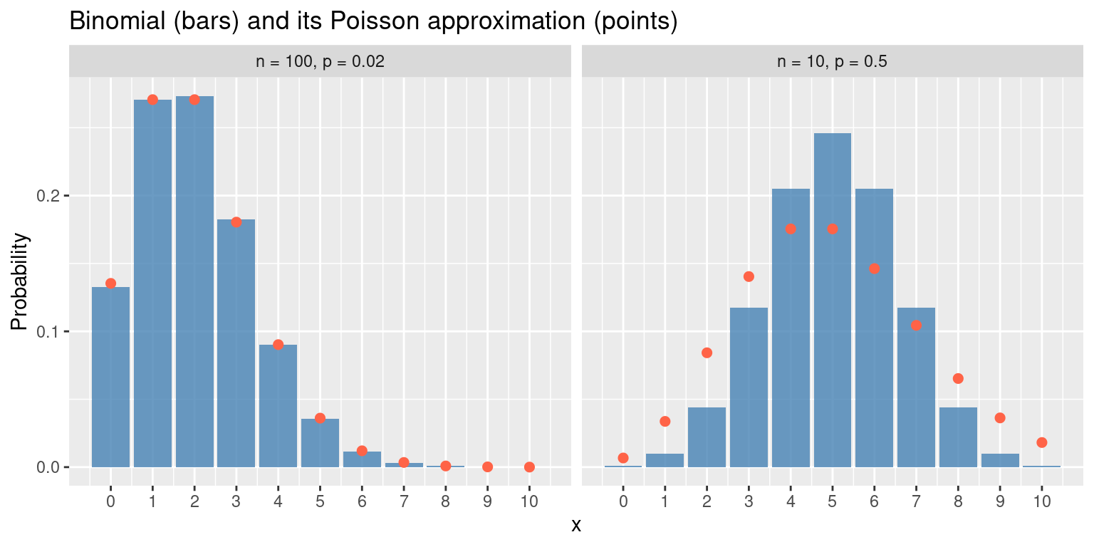
Let’s compare the two distributions for a good case and a bad case. In each panel the bars are the binomial probabilities and the points are the Poisson approximation with \(\lambda = np\).
library(tidyverse)compare <-function(n, p, xmax) {tibble(x =0:xmax,Binomial =dbinom(x, n, p),Poisson =dpois(x, n * p),case =sprintf("n = %d, p = %s", n, p))}both <-bind_rows(compare(100, 0.02, 10), compare(10, 0.5, 10)) %>%mutate(case =fct_inorder(case))ggplot(both, aes(x)) +geom_col(aes(y = Binomial), fill ="steelblue", alpha =0.8) +geom_point(aes(y = Poisson), colour ="tomato", size =2) +facet_wrap(~ case) +scale_x_continuous(breaks =0:10) +labs(title ="Binomial (bars) and its Poisson approximation (points)",x ="x", y ="Probability")
On the left (\(n = 100\), \(p = 0.02\)) the points sit on top of the bars. On the right (\(n = 10\), \(p = 0.5\)) the Poisson with \(\lambda = 5\) is too spread out and has the wrong shape, because \(p\) is far from small.
How Close Is It? The Largest Error
One number summarises the fit: the largest gap between the two probabilities over all \(x\).
max_gap <-function(n, p) max(abs(dbinom(0:n, n, p) -dpois(0:n, n * p)))tibble(n =c(20, 100, 100, 1000, 10),p =c(0.05, 0.02, 0.01, 0.002, 0.5)) %>%mutate(lambda = n * p,max_gap =round(map2_dbl(n, p, max_gap), 5))
For the rare-event cases the largest gap is tiny, and it shrinks further as \(n\) grows with \(\lambda\) fixed. For \(n = 10\), \(p = 0.5\) the gap is large, so we should not use the approximation there.
Fixed n, Changing p
Two summaries measure the difference over all values of \(x\):
the largest gap between the two probabilities, and
The total variation distance is the largest error we can make in the probability of any event, so it is the more honest summary. (The Poisson mass beyond \(x = n\) is included.)
gap_table <-function(n, p) {tibble(n = n, p = p) %>%mutate(lambda = n * p,max_gap =map2_dbl(n, p, max_gap),tv_dist =map2_dbl(n, p, function(n, p)0.5* (sum(abs(dbinom(0:n, n, p) -dpois(0:n, n * p))) +ppois(n, n * p, lower.tail =FALSE)))) %>%mutate(across(c(max_gap, tv_dist), ~round(.x, 5)))}knitr::kable(gap_table(n =100, p =c(0.01, 0.02, 0.05, 0.1, 0.2, 0.5)))
n
p
lambda
max_gap
tv_dist
100
0.01
1
0.00185
0.00278
100
0.02
2
0.00274
0.00457
100
0.05
5
0.00455
0.01260
100
0.10
10
0.00676
0.02583
100
0.20
20
0.01046
0.05416
100
0.50
50
0.02326
0.16662
With \(n = 100\) fixed, both measures grow as \(p\) grows. At \(p = 0.01\) the approximation is excellent. By \(p = 0.5\) it is poor, even though \(n\) is large, which shows that a small \(p\), not just a large \(n\), is what matters.
Fixed p, Changing n
Now we fix \(p = 0.02\) and let \(n\) grow.
knitr::kable(gap_table(n =c(10, 20, 50, 100, 500, 1000), p =0.02))
n
p
lambda
max_gap
tv_dist
10
0.02
0.2
0.00300
0.00300
20
0.02
0.4
0.00437
0.00437
50
0.02
1.0
0.00372
0.00558
100
0.02
2.0
0.00274
0.00457
500
0.02
10.0
0.00127
0.00494
1000
0.02
20.0
0.00090
0.00487
Now the two measures behave differently. The largest gap shrinks as \(n\) increases, because the probability is spread over more values of \(x\). The total variation distance does not shrink: it levels off at a small value close to \(0.005\). It cannot exceed \(p\) (a known bound), so the error of the approximation is controlled mainly by \(p\), however large \(n\) is.
So a larger \(n\) alone does not make the approximation better. A small \(p\) is what makes it good, and a large \(n\) then lets us use it for a wide range of counts.
Tip
Why bother, when software computes exact binomial probabilities? Historically the Poisson formula was far easier to calculate by hand, and it still gives a clear interpretation: a count of rare events with an average rate \(\lambda\).
Summary
Use \(B(n, p) \approx P(np)\) when \(n\) is large and \(p\) is small.
Rule of thumb: \(n \ge 20\) and \(p \le 0.05\), and better with \(n \ge 100\) and \(p \le 0.01\).
Check the fit by comparing the probabilities, as in the examples above.