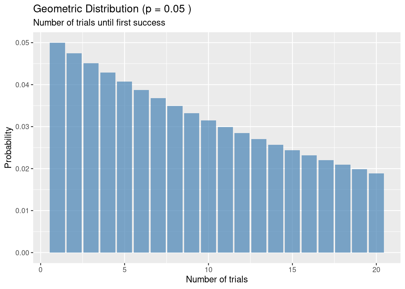
The geometric distribution models the number of trials until the first success in independent Bernoulli trials. This post explains when and why to use it, with a real-world example and R visualization.
probability
discrete distributions
Author
Abdullah Al Mahmud
Published
August 5, 2026
What is the Geometric Distribution?
The geometric distribution models the number of trials needed to get the first success in a sequence of independent Bernoulli trials (each with success probability \(p\)).
It answers questions like: “How many times must we try before we succeed for the first time?”
Key Characteristics
Memoryless property: The probability of success in the next trial does not depend on how many failures have already occurred.
Two common formulations:
Version
What it models
PMF
Support
Type 1
Number of trials until first success (including the success)
\(P(X = k) = (1-p)^{k-1}p\)
\(k = 1, 2, 3, \dots\)
Type 2
Number of failures before first success
\(P(Y = y) = (1-p)^y p\)
\(y = 0, 1, 2, \dots\)
Real-World Example
A quality control inspector tests items coming off an assembly line. Each item has a 5% chance of being defective. What is the probability that the first defect is found on the 5th item tested?
library(ggplot2)p <-0.05x <-1:20prob <-dgeom(x -1, p) # Type 1: P(X = k) = (1-p)^(k-1) pdf <-data.frame(Trials = x, Probability = prob)ggplot(df, aes(x = Trials, y = Probability)) +geom_col(fill ="steelblue", alpha =0.7) +labs(title =paste("Geometric Distribution (p =", p, ")"),subtitle ="Number of trials until first success",x ="Number of trials", y ="Probability")