Reading a Frequency Distribution: Insights from a Histogram and Polygon

Histogram bars for commute-time classes from 10 to 60 minutes with a blue frequency polygon peaking in the 30 to 40 minute class. — A histogram of commute times with a frequency polygon joining the class midpoints.

To see how a frequency distribution and a histogram work in practice, let’s use a continuous dataset: the daily one-way commute times of employees at a large office.

The Dataset: Daily Commute Times

Suppose we surveyed 200 employees. Their commute times (in minutes) give this frequency distribution:

Commute time (min)	Employees	Typical commute
10–20	25	Short, local
20–30	60	Standard city transit or driving
30–40	70	Most common; typical suburban commute
40–50	30	Longer, some traffic
50–60	15	Heavy traffic or distant suburbs

Visualizing the Distribution

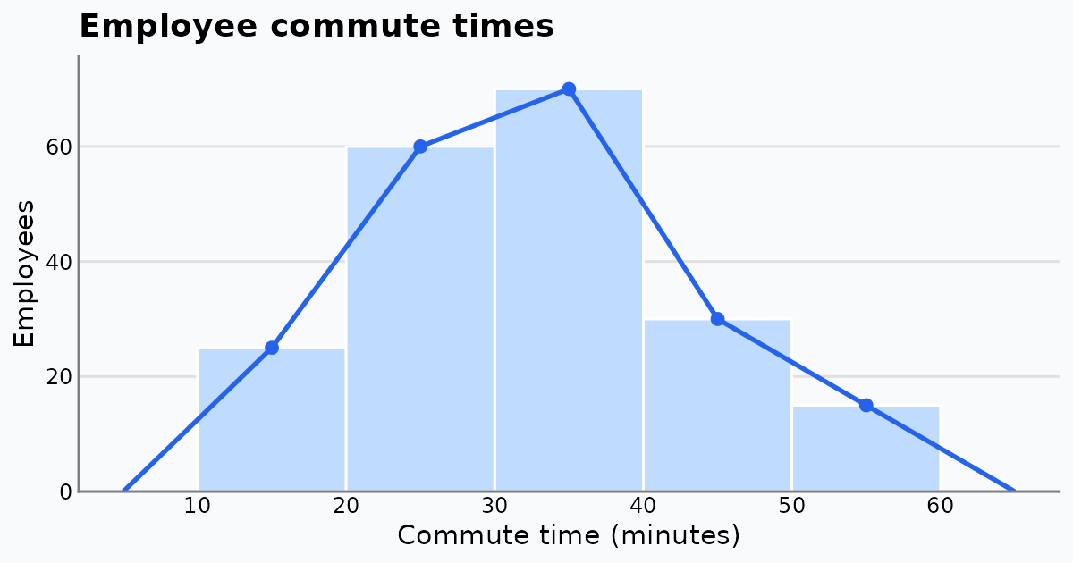
We plot the table as a histogram (bars) with a frequency polygon (a line joining the class midpoints). The polygon is closed at both ends with an empty class of frequency 0.

library(ggplot2)

commute <- data.frame(
  interval  = c("10–20", "20–30", "30–40", "40–50", "50–60"),
  midpoint  = c(15, 25, 35, 45, 55),
  employees = c(25, 60, 70, 30, 15)
)

# polygon points: add an empty class at each end
polygon_pts <- rbind(
  data.frame(midpoint = 5,  employees = 0),
  commute[, c("midpoint", "employees")],
  data.frame(midpoint = 65, employees = 0)
)

ggplot(commute, aes(midpoint, employees)) +
  geom_col(width = 10, fill = "#375faf", colour = "#5b7cbd") +
  geom_line(data = polygon_pts, colour = "#002266", linewidth = 1) +
  geom_point(colour = "#002266", size = 2.5) +
  geom_text(aes(label = employees), vjust = -0.8) +
  scale_x_continuous(breaks = seq(10, 60, 10)) +
  scale_y_continuous(limits = c(0, 80), expand = c(0, 0)) +
  labs(title = "Daily commute times of 200 employees",
       x = "Commute time (minutes)", y = "Number of employees") +
  theme(axis.ticks = element_blank())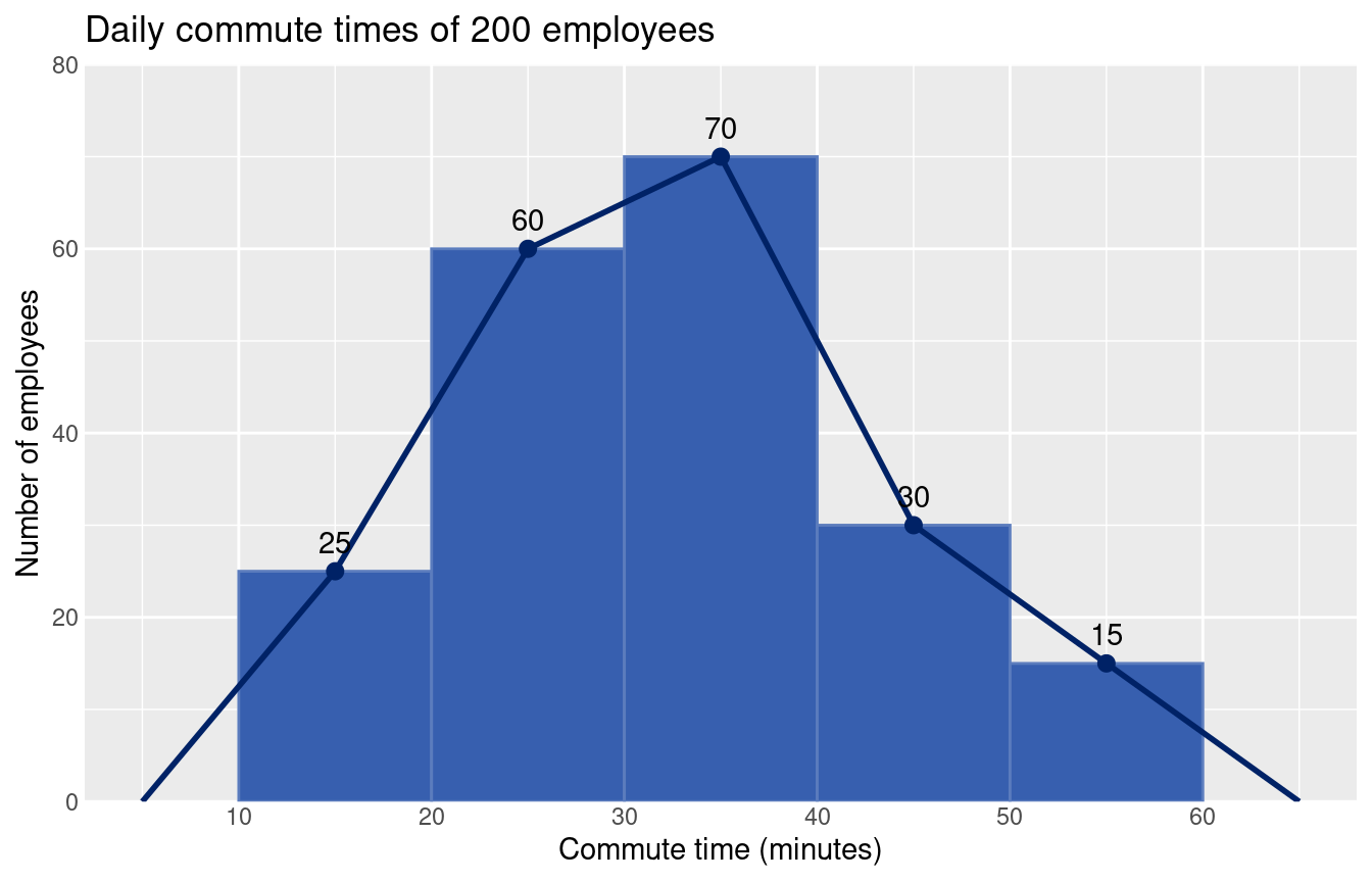

Key Insights

Mode: the 30–40 minute class is the largest (70 employees). The polygon peaks at its midpoint, 35 minutes, so a commute of about 35 minutes is the most common.
Shape: the distribution is roughly symmetric around that peak. The mean and median, computed below, are close to each other.
Concentration: 130 of the 200 employees (65%) travel 20–40 minutes. That range is a sensible baseline for thinking about core hours or hybrid-work policy.

We can check these numbers from the frequency table:

n <- sum(commute$employees)

# mean from class midpoints
mean_est <- sum(commute$midpoint * commute$employees) / n

# median by interpolation inside the median class (30-40)
cum_before <- sum(commute$employees[1:2])      # employees below 30
median_est <- 30 + (n / 2 - cum_before) / 70 * 10

# share in the 20-40 minute range
share <- sum(commute$employees[2:3]) / n

c(n = n, mean = mean_est, median = median_est, share_20_40 = share)

          n        mean      median share_20_40 
  200.00000    32.50000    32.14286     0.65000

Histogram vs Polygon: What Each Shows

Histogram bars show how much data sits in each class. The 20–30 and 30–40 bars clearly hold most employees.
Frequency polygon smooths the hard class edges and shows the shape of the rise and fall. It would also let us overlay a second office on the same axes and compare the two commute profiles easily.

See Frequency Polygons and Frequency Curves for more on when to use each chart.