Is the Poisson Distribution Memoryless? Poisson vs Exponential
Strictly, no: the memoryless property belongs to the exponential waiting time between Poisson events, not to the Poisson count. We define the property, compare the two distributions, and check it numerically in R.
R
Statistics
Probability
Author
Abdullah Al Mahmud
Published
November 4, 2026
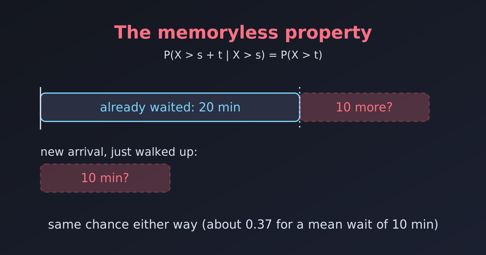
A bus that never gets “due”: the wait to the next event ignores how long we have already waited.
A waiting time is memoryless if how long we have already waited tells us nothing about how much longer we will wait. Think of waiting for a random event, such as a call or a bus: after 20 minutes of waiting, we are no closer to the event than when we started. Does the Poisson distribution have this property?
Strictly speaking, the Poisson distribution itself is not memoryless. What is memoryless is the exponential distribution of the waiting time between events in a Poisson process. The two are closely linked, which is why they get confused. Let’s separate them.
What the Memoryless Property Means
A waiting time \(X\) is memoryless if the past does not change the chance of a future outcome:
\[
P(X > s + t \mid X > s) = P(X > t).
\]
\(s\) is the time we have already waited.
\(t\) is the additional time we are asking about.
In plain words: if we have waited \(s\) minutes and nothing has happened, the probability of waiting at least \(t\) more minutes is exactly what it would be for someone who has just arrived. The process “forgets” how long it has run.
Poisson Count vs Exponential Waiting Time
Poisson
Exponential
What it models
The number of events in a fixed interval
The waiting time between events
Type of variable
Discrete (0, 1, 2, …)
Continuous (\(x > 0\))
Example
Emails arriving in an hour
Minutes between one email and the next
Memoryless?
No
Yes, and it is the only continuous distribution that is
The Poisson process has independent increments: counts in non-overlapping time windows do not affect each other. That is a different idea from memorylessness, which is a property of one waiting time.
If events arrive as a Poisson process with rate \(\lambda\), the counts in a unit interval are Poisson(\(\lambda\)), and the waiting times between events are exponential with the same rate \(\lambda\).
Checking the Memoryless Property in R
For an exponential waiting time, the probability of waiting longer than \(x\) is \(e^{-\lambda x}\). Let’s take a rate of \(\lambda = 0.1\) events per minute (one event every 10 minutes on average), and ask: having waited \(s = 20\) minutes, what is the chance of waiting at least \(t = 10\) more?
rate <-0.1s <-20t <-10# P(X > s + t | X > s) = P(X > s + t) / P(X > s)pexp(s + t, rate, lower.tail =FALSE) /pexp(s, rate, lower.tail =FALSE)
[1] 0.3678794
# P(X > t), for someone who has just arrivedpexp(t, rate, lower.tail =FALSE)
[1] 0.3678794
The two numbers are identical, \(e^{-1} \approx 0.368\). We can also check it by simulation, using only the waits that already exceeded \(s\):
set.seed(1)waits <-rexp(1e6, rate)mean(waits[waits > s] > s + t) # among those who waited s, share who waited t more
[1] 0.3676605
mean(waits > t) # share of all waits longer than t
[1] 0.368468
Both are about \(0.37\), as the property says.
A Waiting Time That Is Not Memoryless
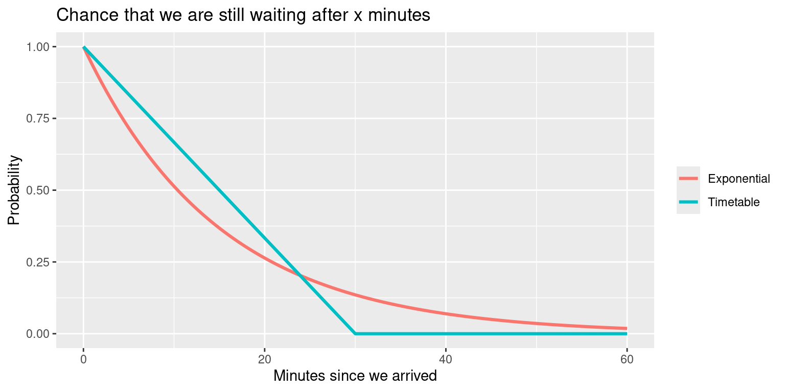
For contrast, think of a bus that comes on a timetable, every 30 minutes. If we arrive at a random moment, the wait is uniform from 0 to 30 minutes. Now the past matters.
library(tidyverse)wait <-seq(0, 60, by =0.5)curves <-tibble(minutes = wait,Exponential =pexp(wait, 1/15, lower.tail =FALSE),Timetable =punif(wait, 0, 30, lower.tail =FALSE)) %>%pivot_longer(-minutes, names_to ="bus", values_to ="chance_still_waiting")ggplot(curves, aes(minutes, chance_still_waiting, colour = bus)) +geom_line(linewidth =1.1) +labs(title ="Chance that we are still waiting after x minutes",x ="Minutes since we arrived", y ="Probability", colour =NULL)
For the timetable bus, once we have waited 20 minutes the bus is certain to come within 10 more. A new arrival could wait up to 30. The wait does depend on the past. For the exponential bus, the chance of waiting \(t\) more minutes is the same no matter how long we have already waited.
Example: The Bus at a Random Stop
Suppose buses at a stop arrive at random, as a Poisson process, with \(\lambda = 0.1\) per minute.
If we have already waited 20 minutes, the chance that we wait at least 10 more is \(e^{-1} \approx 0.368\).
A new passenger who has just walked up has exactly the same \(0.368\) chance of waiting at least 10 minutes.
The bus does not become “due” because we have waited longer, and the process does not accumulate wear or memory.
Note
This is why waiting for a random event is frustrating. It is not that a long wait makes the event more likely. For truly random arrivals, the future is the same however long we have waited. A timetable is different, because there the past does carry information.
Summary
The Poisson distribution counts events in an interval, and is not memoryless.
The exponential distribution models the waiting time between those events, and is memoryless: \(P(X > s + t \mid X > s) = P(X > t)\).
It is the only continuous distribution with this property.