library(tidyverse)

set.seed(2026)
n <- 2000

points <- tibble(
  x = runif(n, -1, 1),
  y = runif(n, -1, 1)
) %>%
  mutate(inside = x^2 + y^2 <= 1)

4 * mean(points$inside)
[1] 3.172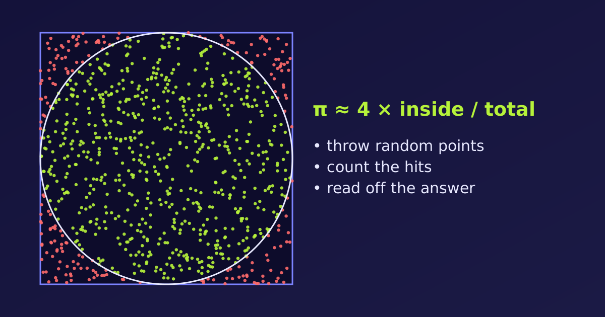
Some problems are too messy for a neat formula: the chance that a portfolio crashes, the path of a particle through a material, the best move in a board game. The Monte Carlo method solves them by brute-force randomness. We simulate the situation many times with random inputs, and read the answer off the results. Let’s see the idea on the simplest example, and then build it in R.
A Monte Carlo method estimates a quantity by repeating a random experiment many times and averaging what happens. The name comes from the Monte Carlo casino in Monaco, a nod to the role of chance. The recipe has the same four steps every time:
It works because of the law of large numbers: the more random samples we use, the closer their average gets to the true value. The error shrinks roughly like \(1/\sqrt{n}\), so ten times the accuracy costs a hundred times the samples. This is slow, but it works for almost any problem, however complicated.
Imagine a perfectly round circle drawn inside a square on a wall. We want the area of the circle, but we pretend we do not know its formula. So we play a game:
If 785 of 1,000 splatters land inside the circle, the circle covers about 78.5% of the square. Since the square’s area is easy (width × height), the circle’s area is that area times 0.785.
Take a square from \(-1\) to \(1\) on both axes, with a circle of radius 1 inside it. The square has area \(2 \times 2 = 4\) and the circle has area \(\pi r^2 = \pi\). So the share of points inside the circle should be \(\pi / 4\), which gives
\[\pi \approx 4 \times \frac{\text{points inside the circle}}{\text{total points}}.\]
A point \((x, y)\) is inside the circle when \(x^2 + y^2 \le 1\).
library(tidyverse)
set.seed(2026)
n <- 2000
points <- tibble(
x = runif(n, -1, 1),
y = runif(n, -1, 1)
) %>%
mutate(inside = x^2 + y^2 <= 1)
4 * mean(points$inside)[1] 3.172runif() draws uniform random numbers, and mean() of a logical column is the share of TRUE values, so 4 * mean(inside) is exactly the formula above. The true value is 3.1416.
circle <- tibble(t = seq(0, 2 * pi, length.out = 300)) %>%
  mutate(x = cos(t), y = sin(t))

ggplot(points, aes(x, y, colour = inside)) +
  geom_point(size = 1) +
  geom_path(data = circle, aes(x, y), colour = "black", inherit.aes = FALSE) +
  coord_fixed() +
  scale_colour_manual(values = c("TRUE" = "seagreen", "FALSE" = "tomato"),
                      labels = c("TRUE" = "Inside", "FALSE" = "Outside")) +
  labs(title = "2000 random points in the square", colour = NULL)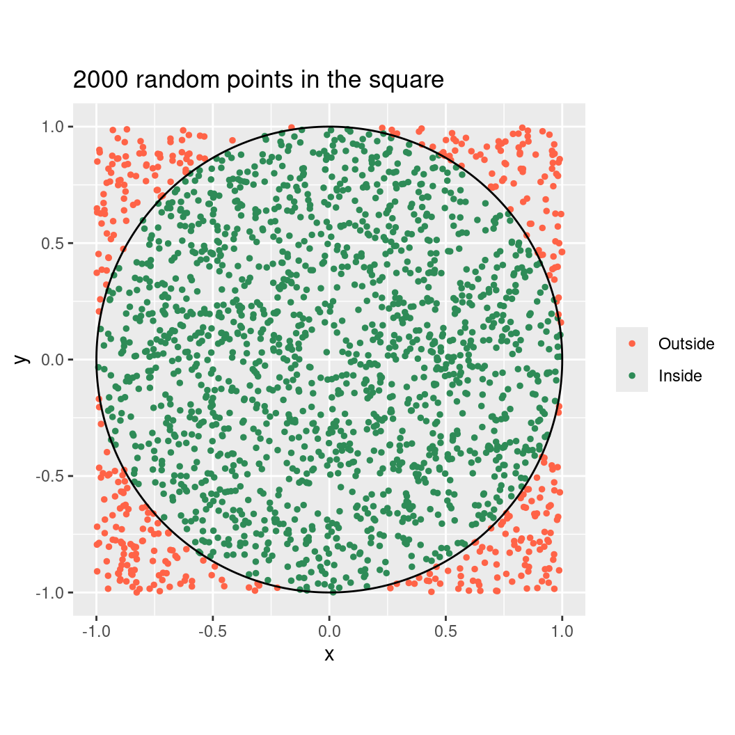
The green points inside the circle make up about \(\pi/4 \approx 78.5\%\) of all points.
How many points do we need? Let’s keep a running estimate as the points arrive and plot it.
set.seed(2026)
N <- 100000

running <- tibble(
  n = 1:N,
  inside = runif(N, -1, 1)^2 + runif(N, -1, 1)^2 <= 1
) %>%
  mutate(estimate = 4 * cumsum(inside) / n)

ggplot(running, aes(n, estimate)) +
  geom_line(colour = "steelblue") +
  geom_hline(yintercept = pi, colour = "tomato", linetype = "dashed") +
  scale_x_log10(labels = scales::comma) +
  labs(title = "The estimate settles down as n grows",
       x = "Number of points (log scale)", y = "Estimate of π")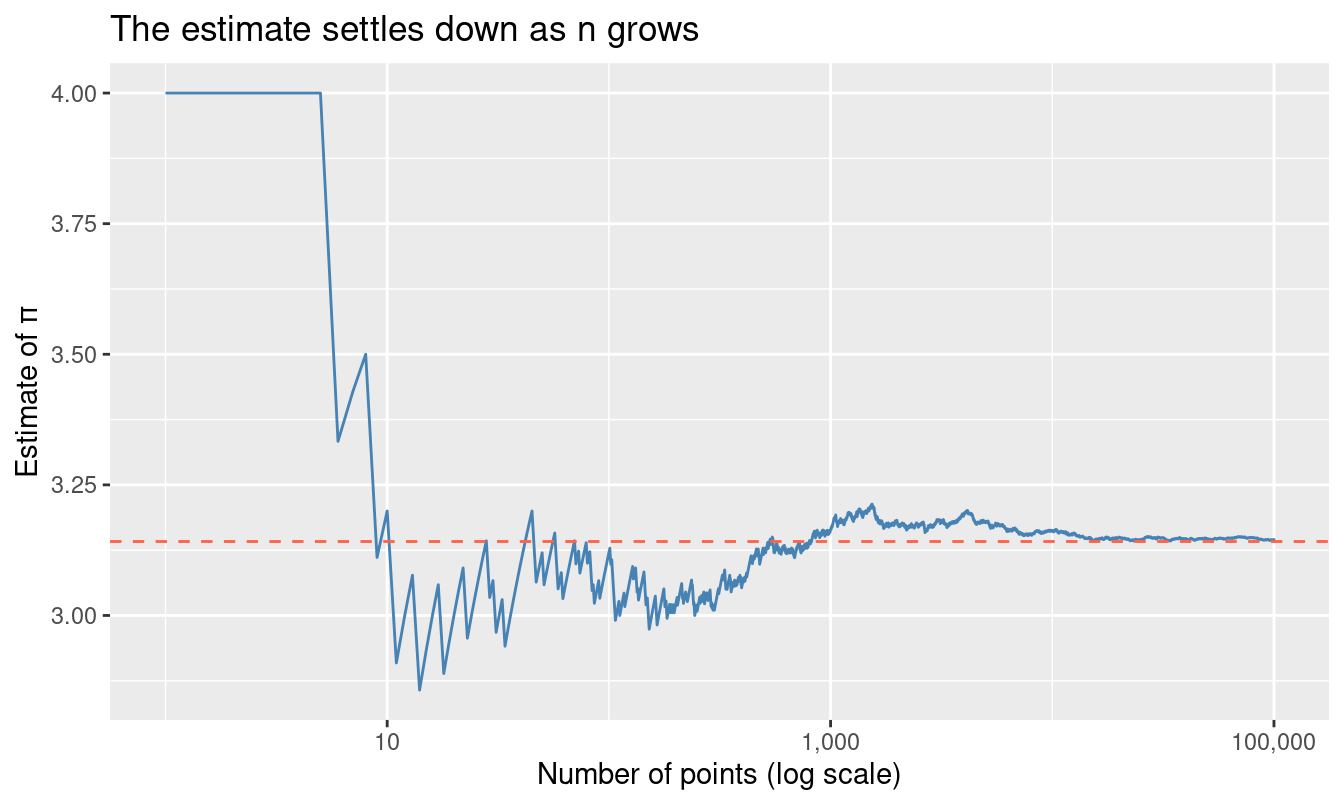
At the start the line jumps around, which is the “pure luck” of few throws. After a few thousand points it hugs the dashed line at \(\pi\). A table shows the same story:
running %>%
  filter(n %in% c(10, 100, 1000, 10000, 100000)) %>%
  transmute(n, estimate = round(estimate, 4), error = round(abs(estimate - pi), 4))
# A tibble: 5 × 3
n estimate error
<int> <dbl> <dbl>
1 10 3.2 0.0584
2 100 3.12 0.0216
3 1000 3.16 0.0224
4 10000 3.16 0.02
5 100000 3.15 0.0036The error shrinks as \(n\) grows, though not steadily: a lucky small sample can beat an unlucky larger one.
Run the code again with a different set.seed(). The numbers change, but the pattern (wild at first, then steady) does not. That is the Monte Carlo method at work.
Computers use this “dirt-throwing” logic to simulate millions of random scenarios in seconds. It is used when the problem is too complex for a straight formula:
Estimating π is not a good use of Monte Carlo, since much better methods exist. We use it because we know the answer, which lets us watch the method work.