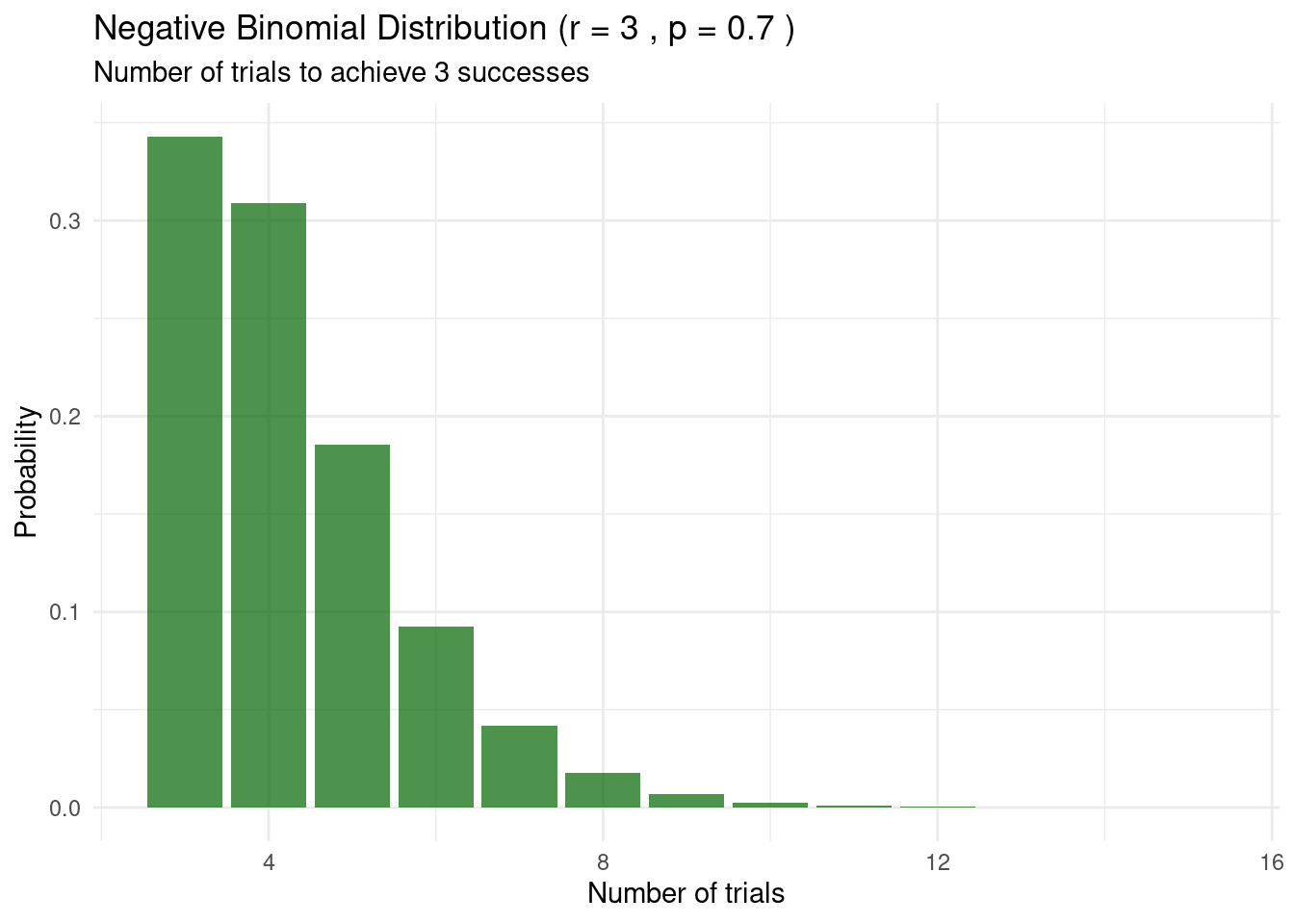
The negative binomial distribution models the number of trials needed to achieve a fixed number of successes. This post explains its formulation, real-world applications, and provides a visual example.
probability
discrete distributions
Author
Abdullah Al Mahmud
Published
May 12, 2026
Description
The negative binomial distribution is a discrete probability distribution that models the number of trials required to obtain a fixed number of successes (\(r\)) in a sequence of independent Bernoulli trials, each with success probability \(p\).
It generalizes the geometric distribution (which is the special case where \(r = 1\), i.e., waiting for the first success).
Probability Mass Function (PMF)
Two common formulations:
Type
What it models
PMF
Support
Trials until \(r\)-th success
Number of trials needed to get \(r\) successes
\(P(X = k) = \binom{k-1}{r-1} p^r (1-p)^{k-r}\)
\(k = r, r+1, r+2, \dots\)
Number of failures before \(r\)-th success
Number of failures before the \(r\)-th success
\(P(Y = y) = \binom{y+r-1}{r-1} p^r (1-p)^y\)
\(y = 0, 1, 2, \dots\)
Here, the negative binomial can be seen as a sum of \(r\) independent geometric random variables.
Key Properties
Mean (trials formulation): \(E[X] = \frac{r}{p}\)
Mean (failures formulation): \(E[Y] = \frac{r(1-p)}{p}\)
Variance (same for both formulations, since \(X = Y + r\)): \(Var(X) = Var(Y) = \frac{r(1-p)}{p^2}\)
Overdispersion: Comparing against the failures count \(Y\) — the formulation analogous to a Poisson count — the variance exceeds the mean whenever \(p < 1\), i.e. \(\frac{Var(Y)}{E[Y]} = \frac{1}{p} > 1\). This is why the negative binomial suits count data with extra variability (unlike the Poisson distribution, where variance always equals the mean). Note this comparison does not hold for the trials count \(X\) itself — \(Var(X) > E[X]\) only when \(p < 0.5\).
Categories of Use Cases
The negative binomial distribution is widely used in:
Epidemiology – number of contacts until a certain number of disease transmissions occur
Insurance / Actuarial Science – number of claims until a fixed number of payouts
Sports Analytics – number of at‑bats until a player gets a certain number of hits
Manufacturing – number of items produced until a fixed number of defects are found
Machine Learning – modeling overdispersed count data (e.g., number of website visits per user)
Real-World Example
A basketball player has a free‑throw success probability of \(p = 0.70\). What is the probability that she makes her 3rd successful free throw on her 6th attempt?
library(ggplot2)# Parametersr <-3# number of successesp <-0.7# success probabilityk <-3:15# possible number of trials# Probability mass function using dnbinom (failures formulation)# Convert to trials: number of failures = k - rprob <-dnbinom(k - r, size = r, prob = p)# Create data framedf <-data.frame(Trials = k, Probability = prob)# Plotggplot(df, aes(x = Trials, y = Probability)) +geom_col(fill ="darkgreen", alpha =0.7) +labs(title =paste("Negative Binomial Distribution (r =", r, ", p =", p, ")"),subtitle ="Number of trials to achieve 3 successes",x ="Number of trials", y ="Probability") +theme_minimal()
Comparison with Poisson Distribution
All rows below use the failures formulation (\(Y\) = number of failures before the \(r\)-th success), since that is the count analogous to a Poisson-distributed count.
Feature
Negative Binomial
Poisson
Mean
\(\frac{r(1-p)}{p}\)
\(\lambda\)
Variance
\(\frac{r(1-p)}{p^2}\)
\(\lambda\)
Variance / Mean
\(\frac{1}{p} > 1\)
\(1\)
Overdispersion
✅ Handles
❌ Assumes variance = mean
Thus, the negative binomial is often used as a robust alternative to the Poisson when count data exhibit overdispersion.
Key Takeaway
Use the negative binomial distribution when you want to model the number of trials needed to achieve a fixed number of successes, or when count data show more variability than a Poisson would allow. It is a flexible tool for overdispersed counts in real-world applications.