Stem-and-Leaf Plot vs Histogram: Differences, with R Examples

How stem-and-leaf plots and histograms are alike and how they differ: exact values versus counts, small versus large datasets, finding the median. Worked in R with stem() and ggplot2.
R
Statistics
Visualization
Author

Abdullah Al Mahmud

Published

November 2, 2026

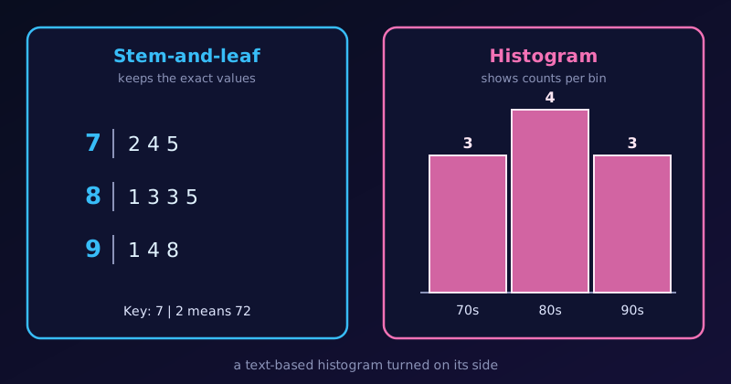
A stem-and-leaf plot of ten scores beside a histogram of the same scores with bars of height 3, 4 and 3.

The same ten scores as a stem-and-leaf plot and as a histogram.

Stem-and-leaf plots and histograms both show the distribution of quantitative data. A stem-and-leaf plot is often described as a text-based histogram turned on its side. They serve slightly different purposes, depending on the size of the dataset and what we want to emphasise.

How They Are Similar

  1. They show the shape of the data. We can see whether the data are symmetric, skewed to the left or right, or have several peaks.
  2. They group data into intervals. A histogram calls them bins (such as 70–79). A stem-and-leaf plot uses the stems (such as the tens digit).
  3. They display frequency. In a histogram it is the height of a bar; in a stem-and-leaf plot it is the length of a row of leaves.
  4. They are for quantitative data. Neither suits categories such as eye colour or car brand.

How They Differ

Feature Stem-and-leaf plot Histogram
Data retention Keeps the exact values in the leaves Loses the exact values: a bar only gives a count
Visual format Digits form the “bars” Solid rectangular bars
Class intervals Set by place value (tens, hundreds, …) Bin width chosen freely
Dataset size Small to medium (about 15–50 values) Large (hundreds or thousands)
Finding the median Easy: count to the middle leaf Harder: estimate inside a bar
Ordering Sorted leaves give the exact rank of every value Individual points are lost, so no exact rank

An Example with Ten Scores

Here are ten test scores:

scores <- c(72, 74, 75, 81, 83, 83, 85, 91, 94, 98)

As a stem-and-leaf plot

stem(scores)
  The decimal point is 1 digit(s) to the right of the |

  7 | 245
  8 | 1335
  9 | 148

Key: 7 | 2 means 72. We can read every score, see that the most common one is 83, and find the median by counting to the middle:

median(scores)
[1] 83

As a histogram

library(ggplot2)

scores <- c(72, 74, 75, 81, 83, 83, 85, 91, 94, 98)

ggplot(data.frame(scores), aes(scores)) +
  geom_histogram(binwidth = 10, boundary = 70, closed = "left",
                 fill = "steelblue", colour = "white") +
  stat_bin(binwidth = 10, boundary = 70, closed = "left",
           geom = "text", aes(label = after_stat(count)), vjust = -0.5) +
  scale_x_continuous(breaks = seq(70, 100, 10)) +
  scale_y_continuous(limits = c(0, 5), expand = c(0, 0)) +
  labs(title = "Histogram of ten test scores",
       x = "Score", y = "Frequency") +
  theme_classic(base_size = 13) +
  theme(axis.ticks = element_blank(),
        axis.line = element_line(colour = "grey60"),
        panel.grid.major.y = element_line(colour = "grey90"))

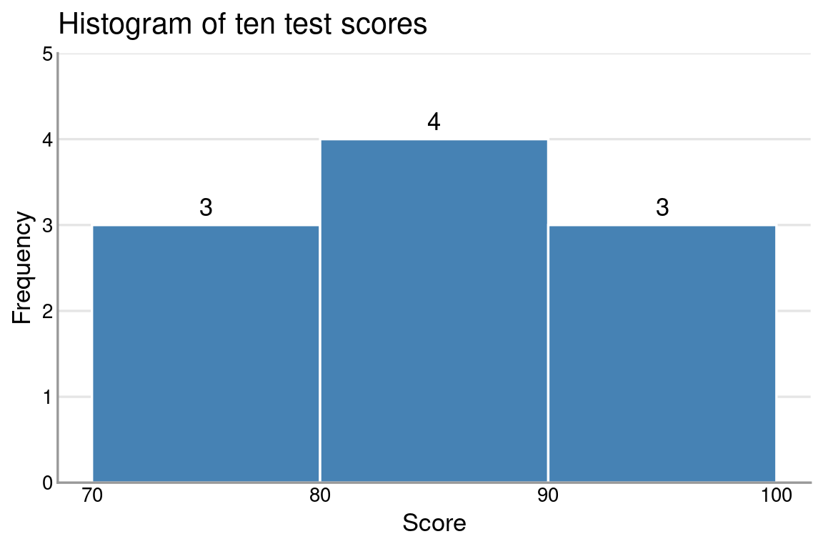
The histogram gives the general shape and the counts (3, 4 and 3). But if we ask “did anyone score 85?”, the bars cannot tell us. The stem-and-leaf plot can: there is an 8 | 5.

When the Dataset Gets Large

With a few dozen values the stem-and-leaf plot is compact. With hundreds, the rows of leaves become very long. Here are 200 simulated scores:

set.seed(7)
big <- round(rnorm(200, mean = 70, sd = 12))

stem(big)

  The decimal point is 1 digit(s) to the right of the |

   4 | 2
   4 | 7789
   5 | 011112223444
   5 | 56677788999999999
   6 | 000001222233333333
   6 | 55555556666667777888889999999
   7 | 0000000111112222222333444444444444444
   7 | 555666666666777777778888888899999999
   8 | 0000011222222233333344444
   8 | 55555666899
   9 | 003
   9 | 667789
  10 | 3

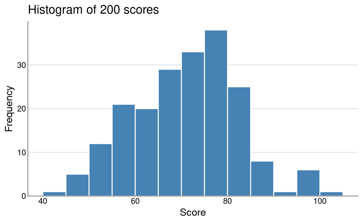
It still works, but the rows are crowded and hard to scan. The histogram handles the same data cleanly:
ggplot(data.frame(big), aes(big)) +
  geom_histogram(binwidth = 5, boundary = 0,
                 fill = "steelblue", colour = "white") +
  scale_y_continuous(expand = expansion(mult = c(0, 0.05))) +
  labs(title = "Histogram of 200 scores",
       x = "Score", y = "Frequency") +
  theme_classic(base_size = 13) +
  theme(axis.ticks = element_blank(),
        axis.line = element_line(colour = "grey60"),
        panel.grid.major.y = element_line(colour = "grey90"))

Summary

  • Use a stem-and-leaf plot for a small dataset when we want to see the shape without losing the original numbers.
  • Use a histogram for a large dataset when only the overall distribution pattern matters.

If a stem-and-leaf plot gives too few rows, see Hybrid Stem-and-Leaf Plot, which uses stems of 5.