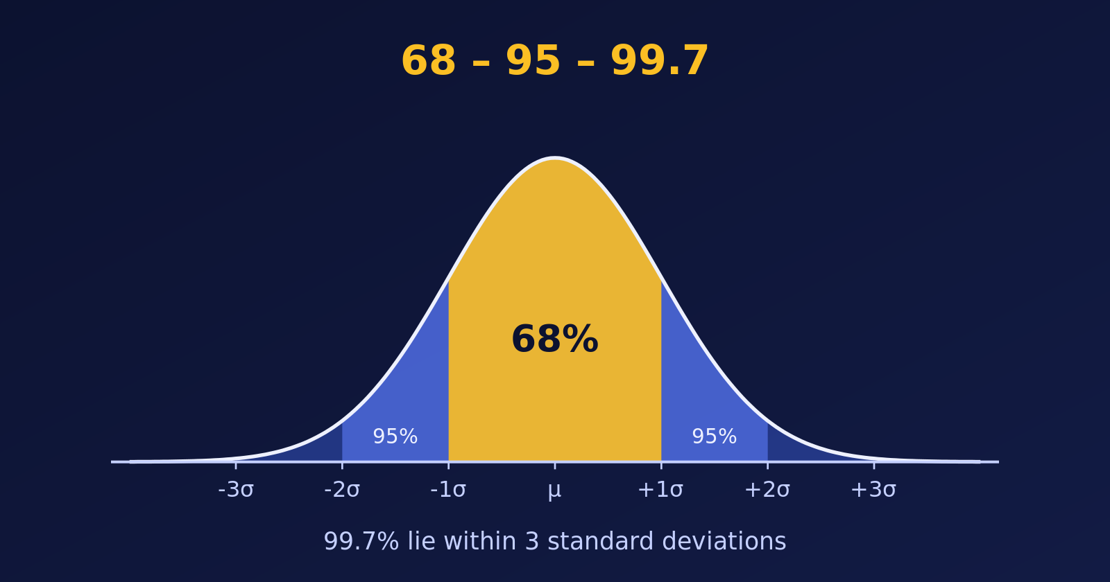
The Empirical Rule says about 68%, 95% and 99.7% of a bell-shaped data set lie within one, two and three standard deviations of the mean. We check it with 10,000 simulated exam scores and draw it with ggplot2.
R
Statistics
Probability
Author
Abdullah Al Mahmud
Published
November 4, 2026
The 68-95-99.7 rule: bands of one, two and three standard deviations around the mean.
The Empirical Rule, also called the 68-95-99.7 rule, tells us how data spread around the mean when the distribution is bell-shaped (normal). Let’s state it, check it with a simulation in R, and then draw it.
An Example First
Suppose the marks of a large group of students are bell-shaped, with a mean of \(\mu = 70\) and a standard deviation of \(\sigma = 5\). The Empirical Rule then says:
about \(68\%\) of the students score within one standard deviation of the mean: between \(\mu - \sigma = 65\) and \(\mu + \sigma = 75\),
about \(95\%\) score within two standard deviations: between \(\mu - 2\sigma = 60\) and \(\mu + 2\sigma = 80\),
about \(99.7\%\), almost everyone, score within three standard deviations: between \(\mu - 3\sigma = 55\) and \(\mu + 3\sigma = 85\).
So a mark below \(55\) or above \(85\) is very unusual: fewer than \(3\) students in \(1{,}000\).
The Empirical Rule
For a normally distributed data set with mean \(\mu\) and standard deviation \(\sigma\):
Range
Share of the data
\([\mu - \sigma, \; \mu + \sigma]\)
about \(68\%\)
\([\mu - 2\sigma, \; \mu + 2\sigma]\)
about \(95\%\)
\([\mu - 3\sigma, \; \mu + 3\sigma]\)
about \(99.7\%\)
So nearly all the data lie within three standard deviations of the mean, and values further away are rare.
Checking the Rule with Simulated Data
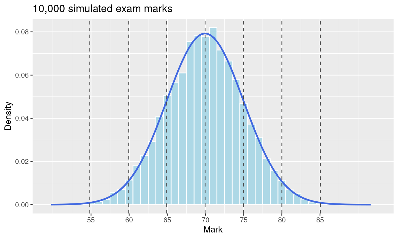
Let’s simulate \(10{,}000\) exam marks like these, with mean \(70\) and standard deviation \(5\), and measure the share of marks within one, two and three standard deviations.
The simulated percentages are very close to the theoretical ones. The theory column is exact: \(68.27\%\), \(95.45\%\) and \(99.73\%\). The familiar \(68\), \(95\) and \(99.7\) are rounded versions of these.
Visualizing the Results
First, the histogram of the scores, with lines at one, two and three standard deviations from the mean.
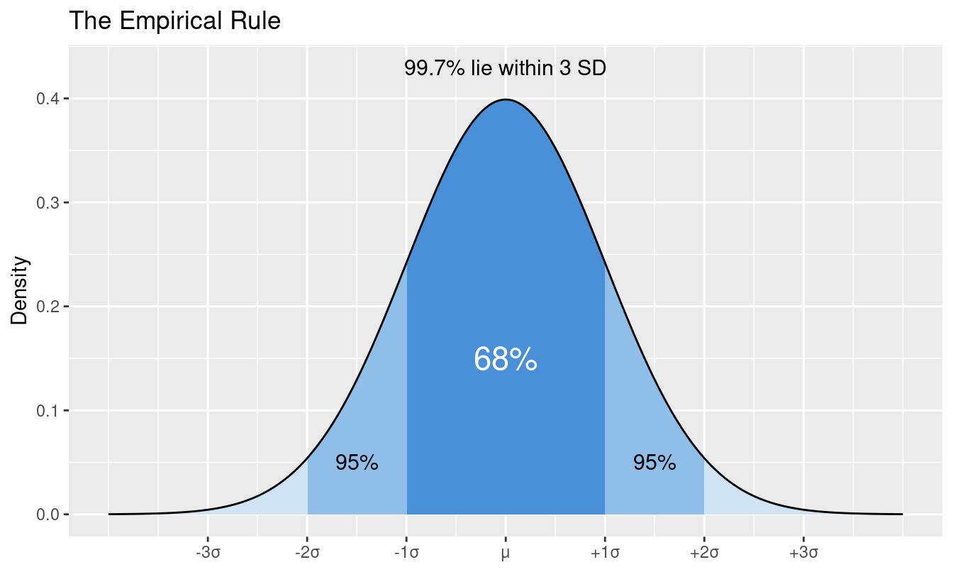
Now the curve itself, with the three bands shaded. The darker the shade, the closer to the mean.
curve <-tibble(x =seq(-4, 4, length.out =800), density =dnorm(x))ggplot(curve, aes(x, density)) +geom_area(fill ="#cfe3f5") +geom_area(data =filter(curve, abs(x) <=2), fill ="#8fbfe8") +geom_area(data =filter(curve, abs(x) <=1), fill ="#4a90d9") +geom_line() +annotate("text", x =0, y =0.15, label ="68%", colour ="white", size =6) +annotate("text", x =1.5, y =0.05, label ="95%", size =4) +annotate("text", x =-1.5, y =0.05, label ="95%", size =4) +annotate("text", x =0, y =0.43, label ="99.7% lie within 3 SD", size =4) +scale_x_continuous(breaks =-3:3, labels =c("-3σ", "-2σ", "-1σ", "μ", "+1σ", "+2σ", "+3σ")) +labs(title ="The Empirical Rule", x =NULL, y ="Density")
The “95%” labels mark the whole region within two standard deviations, which includes the central \(68\%\).
Warning
The rule applies to bell-shaped data. For skewed or heavy-tailed data the percentages can be quite different, so check the shape with a histogram first.
Summary
The Empirical Rule gives \(68\%\), \(95\%\) and \(99.7\%\) for one, two and three standard deviations.
A simulation with rnorm() confirms it: \(68.29\%\), \(95.53\%\) and \(99.73\%\) in our sample.
Shaded areas under the normal curve are the clearest way to show it.