What it says
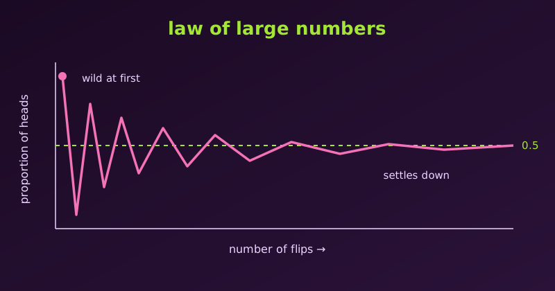
The law of large numbers (LLN) says that as we collect more independent observations from the same distribution, the sample mean gets closer to the true mean:
\[ \bar{X}_n = \frac{X_1 + X_2 + \cdots + X_n}{n} \;\longrightarrow\; \mu \quad \text{as } n \to \infty \]
For a fair coin, let \(X = 1\) for heads and \(0\) for tails. Then \(\mu = 0.5\), and the proportion of heads should approach 0.5 as we flip more.
Seeing it in R
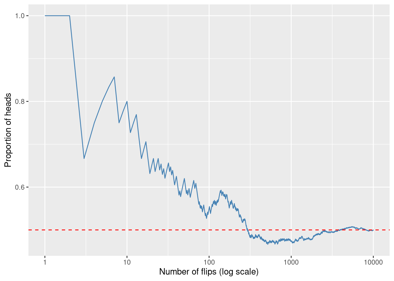
Let’s flip a fair coin 10,000 times and look at the running proportion of heads.
library(ggplot2)

set.seed(42)
n <- 10000
flips <- rbinom(n, 1, 0.5)
running <- cumsum(flips) / seq_len(n)

df <- data.frame(n = seq_len(n), prop = running)

ggplot(df, aes(n, prop)) +
  geom_line(colour = "steelblue") +
  geom_hline(yintercept = 0.5, linetype = "dashed", colour = "red") +
  scale_x_log10() +
  labs(x = "Number of flips (log scale)", y = "Proportion of heads")
The values at a few sample sizes:
      n heads proportion
1    10     8     0.8000
2   100    55     0.5500
3  1000   473     0.4730
4 10000  4999     0.4999
With 10 flips the proportion is far from 0.5; with 10,000 it is very close.
What it is not
1. It is not the gambler’s fallacy
After five heads in a row, tails is not “due”. The coin has no memory, and the next flip is still 50/50. The LLN does not say the past is corrected; it says the early streak gets diluted by the many flips that follow.
2. It does not say counts even out
The proportion approaches 0.5, but the difference between heads and tails does not shrink. It typically grows, like \(\sqrt{n}\). Let’s check by repeating the experiment 5,000 times for each \(n\):
set.seed(1)
sizes <- c(100, 10000, 1000000)
sapply(sizes, function(n) {
  heads <- rbinom(5000, n, 0.5)
  mean(abs(2 * heads - n))
})
n avg_abs_diff avg_prop_off
1 1e+02 8.0 0.07991
2 1e+04 78.2 0.00782
3 1e+06 794.8 0.00079The gap between heads and tails grows from about 8 to about 800, yet as a share of the flips it shrinks toward 0.
3. It is not a promise for small samples
The LLN is a statement about the long run. Ten flips can easily give 8 heads, as in our simulation. Believing that small samples must look like the population is sometimes called the “law of small numbers”, and it is a mistake.
4. It does not make a single outcome predictable
The LLN describes averages over many trials, not the next trial. A casino cannot predict one spin, but it can predict its profit over a million spins.
5. It does not always apply
The LLN needs conditions. The observations should be independent (or weakly dependent) draws from the same distribution, and that distribution must have a finite mean. The Cauchy distribution has no mean, so its sample average never settles, however large \(n\) is.
Note
Don’t confuse the LLN with the central limit theorem. The LLN says the sample mean approaches \(\mu\). The CLT describes the shape of the fluctuations around \(\mu\): roughly normal, with spread \(\sigma / \sqrt{n}\).
A limit that is not the law of large numbers
Not every “settles toward 0.5” story is the LLN. Let’s pick a number \(X\) uniformly from \(1, 2, \dots, n\) with \(n\) odd, and ask for the probability that it exceeds the mean. The mean is \((n+1)/2\), so exactly \((n-1)/2\) of the \(n\) values lie above it:
\[ P(X > \text{mean}) = \frac{n-1}{2n} \]
| \(n\) | 3 | 5 | 11 | 101 | 1001 |
|---|---|---|---|---|---|
| \(P(X > \text{mean})\) | 0.3333 | 0.4000 | 0.4545 | 0.4950 | 0.4995 |
The values creep toward 0.5, but there is no randomness in this table. Each entry is an exact number from algebra, and the limit is the ordinary limit of a sequence.
| This example | Law of large numbers | |
|---|---|---|
| What changes with \(n\) | the distribution itself (more points) | the number of repeated trials of one fixed experiment |
| Randomness | none; exact fixed numbers | each trial is random, so the running average bounces at first |
| Type of convergence | deterministic limit of a sequence of probabilities | the random sample mean approaches \(\mu\) |
| Guarantee | follows from the formula | random fluctuations average out over many trials |
If anything, this example is closer to convergence in distribution: a discrete uniform distribution on \(n\) points, rescaled to \([0, 1]\), approaches the continuous uniform distribution as \(n \to \infty\). The LLN is about something else, namely random sample averages.
Key takeaway
- Large samples give reliable averages, which is why surveys, trials and insurers work.
- The coin never “evens things out”; a larger sample just dilutes early luck.
- The LLN is about the average of many trials, not the next one.