Why Chebyshev’s Inequality Is Great: A Guarantee for Any Distribution

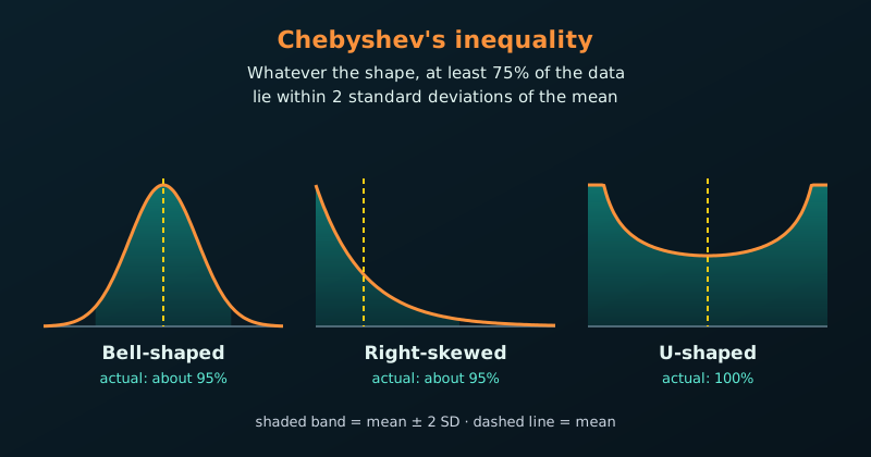
Bell-shaped, right-skewed and U-shaped data: in each, at least 75% lie within two standard deviations of the mean.

Chebyshev’s inequality is great because it guarantees a minimum percentage of data within a certain number of standard deviations from the mean, regardless of the distribution’s shape. We do not need to assume the data follow a Normal bell curve, which makes it a universal safety net for unknown, skewed, or U-shaped datasets.

The Core Formula

For any distribution with a finite mean (\(\mu\)) and finite standard deviation (\(\sigma\)), the proportion of data within \(k\) standard deviations of the mean (\(k > 1\)) is at least

\[ 1-\frac{1}{k^{2}} \]

• Within 2 standard deviations (\(k = 2\)): at least \(1 - \frac{1}{2^2} = 75\%\) of the data.
• Within 3 standard deviations (\(k = 3\)): at least \(1 - \frac{1}{3^2} \approx 88.9\%\) of the data.

Example 1: Heavy-Tailed Data (Household Income)

Income data are skewed to the right because a few very high earners pull the tail far out, so a Normal distribution fits poorly.

Suppose a city reports a mean household income of \(\mu = \$60{,}000\) with a standard deviation of \(\sigma = \$15{,}000\). What is the minimum percentage of households earning between $30,000 and $90,000?

1. Find \(k\). Both boundaries are $30,000 from the mean. Dividing by the standard deviation gives \(k = 30{,}000 / 15{,}000 = 2\).
2. Apply Chebyshev. \(1 - \frac{1}{2^2} = 1 - 0.25 = 0.75\).

Without seeing a single tax return, or knowing the shape of the income gap, we can guarantee that at least 75% of households earn between $30,000 and $90,000.

Example 2: Server Latency and SLA Guarantees

Software response times often follow irregular patterns with random spikes, yet companies must still sign strict Service Level Agreements (SLAs).

Suppose an API has a mean response time of \(\mu = 100\) ms and a standard deviation of \(\sigma = 20\) ms. A client asks for the worst-case share of requests that take 160 ms or longer (or 40 ms or less).

1. Find \(k\). 160 ms is 60 ms from the mean, and \(60 / 20\) gives \(k = 3\).
2. Apply Chebyshev. At least \(1 - \frac{1}{3^2} \approx 88.9\%\) of requests fall between 40 ms and 160 ms. Conversely, at most 11.1% fall outside this range.

Even if network traffic is erratic, the engineers can promise that no more than 11.1% of requests will breach the 160 ms limit (the bound counts both tails, so it is conservative for the slow side alone).

Chebyshev vs. the Normal Distribution

Distance from mean (\(k\))	Normal distribution (bell curve only)	Chebyshev (any distribution)
1.5	86.6%	at least 55.6%
2	95.4%	at least 75.0%
3	99.7%	at least 88.9%
4	99.99%	at least 93.8%

Note

Chebyshev gives a very conservative lower bound. If we know the data are Normal, the Normal distribution gives much tighter estimates.

Testing It in R

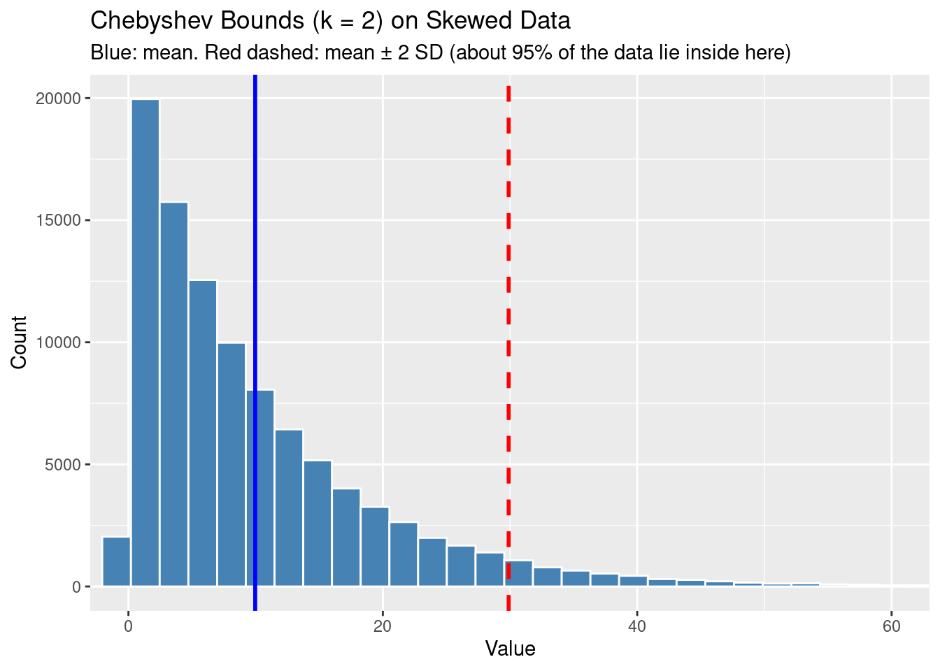
Let’s test the inequality on three very different shapes: a Normal bell curve, a heavily right-skewed Exponential, and a polarised U-shaped Beta (see the U-shaped distribution post). For each, we compute the exact share of data within \(k = 2\) standard deviations of the mean. All three should stay above Chebyshev’s 75% minimum.

set.seed(123)
n <- 100000

# Three completely different distribution shapes
data_normal <- rnorm(n, mean = 50, sd = 10)          # bell-shaped
data_skewed <- rexp(n, rate = 0.1)                   # heavily right-skewed
data_ushape <- rbeta(n, shape1 = 0.5, shape2 = 0.5)  # U-shaped

# Actual % of data within k standard deviations of the mean
check_chebyshev <- function(data, k = 2) {
  mu <- mean(data)
  sigma <- sd(data)
  actual_prop <- mean(data >= mu - k * sigma & data <= mu + k * sigma)
  round(actual_prop * 100, 2)
}

cat("Chebyshev minimum guarantee (k = 2): 75.00%\n")

Chebyshev minimum guarantee (k = 2): 75.00%

cat("Normal distribution actual:        ", check_chebyshev(data_normal), "%\n")

Normal distribution actual:         95.46 %

cat("Right-skewed (Exponential) actual: ", check_chebyshev(data_skewed), "%\n")

Right-skewed (Exponential) actual:  95.08 %

cat("U-shaped (Beta) actual:            ", check_chebyshev(data_ushape), "%\n")

U-shaped (Beta) actual:             100 %

All three comfortably exceed 75%. The bound is a floor valid for every distribution, not a typical value, so real data usually sit well above it.

Visualizing the Bounds

Here are the \(k = 2\) boundaries drawn over the skewed data.

library(ggplot2)

mu_skew <- mean(data_skewed)
sd_skew <- sd(data_skewed)

ggplot(data.frame(x = data_skewed), aes(x)) +
  geom_histogram(bins = 60, fill = "steelblue", colour = "white") +
  geom_vline(xintercept = mu_skew, colour = "blue", linewidth = 1) +
  geom_vline(xintercept = mu_skew + c(-2, 2) * sd_skew,
             colour = "red", linewidth = 1, linetype = "dashed") +
  coord_cartesian(xlim = c(0, 60)) +
  labs(title = "Chebyshev Bounds (k = 2) on Skewed Data",
       subtitle = "Blue: mean. Red dashed: mean ± 2 SD (about 95% of the data lie inside here)",
       x = "Value", y = "Count")

The lower boundary falls below zero, so only the upper line is visible, yet the guarantee still holds.