Double Summation (ΣΣ) in Statistics, and How to Code It in C

A double sum adds each row first, then adds the row totals.

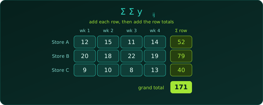
Whenever data sit in a table (groups in rows, observations in columns), we meet the double summation: a sum of sums.

\[ \sum_{i=1}^{a}\sum_{j=1}^{n} y_{ij} \]

Read it from the inside out. For each row \(i\), add the entries \(y_{i1}, \dots, y_{in}\); then add those row totals over \(i = 1, \dots, a\). The result is the grand total of the whole table. The order does not matter for a finite table: summing columns first gives the same number.

Where Statistics Uses It

Quantity	Formula
Grand total	\(\displaystyle \sum_i\sum_j y_{ij}\)
Grand mean	\(\displaystyle \bar y_{..} = \frac{1}{an}\sum_i\sum_j y_{ij}\)
Total sum of squares	\(\displaystyle SST = \sum_i\sum_j \left(y_{ij}-\bar y_{..}\right)^2\)

The total sum of squares is the starting point of one-way ANOVA, which splits it into variation between groups and variation within groups. Chi-square tests, covariance and two-way tables use double sums in the same way.

A Short Real-World Example

A small chain wants to compare three stores. Units sold per week over four weeks:

	Wk 1	Wk 2	Wk 3	Wk 4
Store A	12	15	11	14
Store B	20	18	22	19
Store C	9	10	8	13

How \(i\) and \(j\) Map to the Table

• \(i\) is the row index (the store): \(i = 1\) is Store A, \(i = 2\) is Store B, \(i = 3\) is Store C. So \(a = 3\).
• \(j\) is the column index (the week): \(j = 1, \dots, 4\). So \(n = 4\).
• \(y_{ij}\) is the cell in row \(i\), column \(j\). For example, \(y_{23} = 22\) (Store B, week 3) and \(y_{31} = 9\) (Store C, week 1).

The inner sum fixes a row and runs \(j\) across it:

\[ \sum_{j=1}^{4} y_{1j} = 12 + 15 + 11 + 14 = 52 \]

The outer sum then lets \(i\) move down the rows, adding the row totals:

\[ \sum_{i=1}^{3}\sum_{j=1}^{4} y_{ij} = \underbrace{52}_{i=1} + \underbrace{79}_{i=2} + \underbrace{40}_{i=3} = 171 \]

In words: for each store \(i\), add its four weeks \(j\); then add the three stores.

The row totals are 52, 79 and 40, so the grand total is 52 + 79 + 40 = 171 units, and the grand mean is 171 / 12 = 14.25 units per store-week.

The C Implementation

A double sum is a pair of nested for loops: the outer loop is the outer \(\sum\) (rows) and the inner loop is the inner \(\sum\) (columns). The table is a 2D array, y[i][j].

#include <stdio.h>

#define STORES 3
#define WEEKS  4

int main(void) {
    // y[i][j] = units sold by store i in week j
    int y[STORES][WEEKS] = {
        {12, 15, 11, 14},
        {20, 18, 22, 19},
        { 9, 10,  8, 13}
    };

    // grand total: sum over i, then over j
    int total = 0;
    for (int i = 0; i < STORES; i++) {
        for (int j = 0; j < WEEKS; j++) {
            total += y[i][j];
        }
    }
    double grand_mean = (double)total / (STORES * WEEKS);

    // total sum of squares: SST = sum_i sum_j (y_ij - grand_mean)^2
    double sst = 0.0;
    for (int i = 0; i < STORES; i++) {
        for (int j = 0; j < WEEKS; j++) {
            double d = y[i][j] - grand_mean;
            sst += d * d;
        }
    }

    printf("Grand total     = %d\n", total);
    printf("Grand mean      = %.2f\n", grand_mean);
    printf("Total sum of sq = %.2f\n", sst);
    return 0;
}

Compiled with gcc -Wall -Wextra and run:

Grand total     = 171
Grand mean      = 14.25
Total sum of sq = 232.25

Note

Two details. The sum starts at 0 (the identity for addition), and (double)total converts before dividing; 171 / 12 in integer arithmetic would give 14, not 14.25. We also need the grand mean before the second double sum, which is why the sum of squares is a separate pass.

Summary

Maths	C
\(\sum_i\) (outer sum)	outer for over rows
\(\sum_j\) (inner sum)	inner for over columns
\(y_{ij}\)	y[i][j]
running total	accumulator starting at 0

For more practice with nested loops, see 5 nested for loop practice problems.