Choosing a Chart by Data Type: Categorical, Quantitative or Both

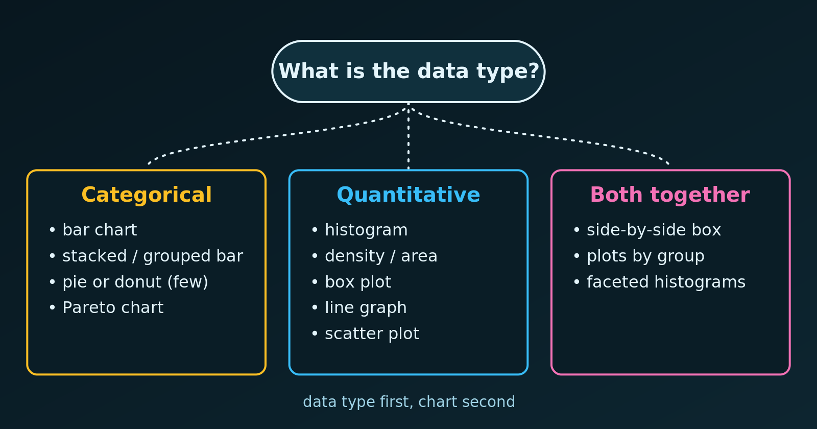
A quick decision guide: the data type points to the chart.

The right chart depends on the type of data in our variables. A wrong choice can distort a relationship, or show data in a way that makes no statistical sense, such as a line graph joining unrelated categories. Let’s go through the three cases and draw an example of each in R.

1. Categorical Data

Categorical (qualitative) data are labels or groups: gender, country, car model, satisfaction level. The usual goal is to compare counts or percentages across groups.

Chart	Best for	Example
Bar chart	Comparing counts or percentages between separate groups	Patients by blood type (\(A\), \(B\), \(AB\), \(O\))
Stacked or grouped bar	A main category split by a second one	Agree / disagree answers by age group
Pie or donut chart	Parts of a whole, with at most about five categories	Market share of a few firms
Pareto chart	Finding the few most frequent categories to prioritise	Frequency of manufacturing defects

2. Quantitative Data

Quantitative (numerical) data are measurable quantities for which arithmetic makes sense. They are either discrete (countable, like shoe sizes or the number of children) or continuous (any value in a range, like height, time or weight).

Chart	Best for	Example
Histogram	The distribution, spread and skewness of one continuous variable	Household incomes in a city
Density or area chart	A smooth distribution, or tail regions	A normal curve and its critical region
Box plot	Five-number summary and outliers	Exam scores in one school
Line graph	A change or trend over time	Global temperature from 1880 to today
Scatter plot	The relationship between two quantitative variables	Hours studied and exam score

3. Mixed Data: Categorical and Quantitative

To see how a number behaves across groups, we use charts that combine both types:

• Side-by-side box plots are the standard way to compare a quantitative variable across categories, for example salary across job titles.
• Faceted histograms show a small histogram for each category, so that we can compare shape, centre and spread.

One Example of Each in R

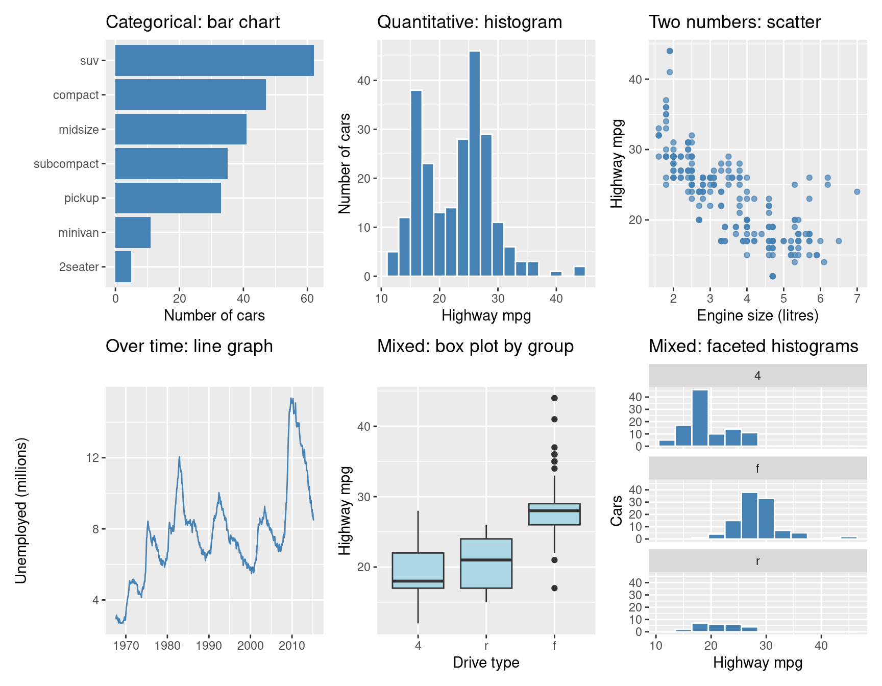
We use the mpg data set that ships with ggplot2 (fuel economy of 234 cars). Each panel matches a row of the tables above. The plots use the default grey panel.

library(ggplot2)
library(patchwork)

bar <- ggplot(mpg, aes(x = reorder(class, class, length))) +
  geom_bar(fill = "steelblue") +
  coord_flip() +
  labs(title = "Categorical: bar chart", x = NULL, y = "Number of cars")

hist <- ggplot(mpg, aes(hwy)) +
  geom_histogram(binwidth = 2, fill = "steelblue", colour = "white") +
  labs(title = "Quantitative: histogram", x = "Highway mpg", y = "Number of cars")

scatter <- ggplot(mpg, aes(displ, hwy)) +
  geom_point(colour = "steelblue", alpha = 0.7) +
  labs(title = "Two numbers: scatter", x = "Engine size (litres)", y = "Highway mpg")

line <- ggplot(economics, aes(date, unemploy / 1000)) +
  geom_line(colour = "steelblue") +
  labs(title = "Over time: line graph", x = NULL, y = "Unemployed (millions)")

box <- ggplot(mpg, aes(x = reorder(drv, hwy, median), y = hwy)) +
  geom_boxplot(fill = "lightblue") +
  labs(title = "Mixed: box plot by group", x = "Drive type", y = "Highway mpg")

facet <- ggplot(mpg, aes(hwy)) +
  geom_histogram(binwidth = 3, fill = "steelblue", colour = "white") +
  facet_wrap(~ drv, ncol = 1) +
  labs(title = "Mixed: faceted histograms", x = "Highway mpg", y = "Cars")

(bar | hist | scatter) / (line | box | facet)

Notice what each chart answers. The bar chart ranks the categories, the histogram shows the shape of one variable, and the scatter plot shows how two variables move together. The line graph follows a change over time, while the box plot and the faceted histograms compare a number across groups.

Common Mistakes

• A line graph for unordered categories. A line suggests a trend between points, so use bars for categories.
• A pie chart with many slices. See pie chart vs bar chart and pie charts with many categories.
• A histogram for categories, or a bar chart for a continuous variable. A histogram’s bars touch because the intervals are continuous, while the bars of a bar chart are separate.

Tip

Ask two questions first: what type is each variable, and what do we want to show (compare, see a distribution, follow a trend, or relate two variables)? The answers almost always point to one chart from the tables above.

Summary

We have	We want	Use
One categorical variable	Compare counts	Bar chart
One categorical variable	Parts of a whole	Pie or donut (few categories)
One quantitative variable	See its distribution	Histogram or box plot
Two quantitative variables	See a relationship	Scatter plot
A quantitative variable over time	See a trend	Line graph
Quantitative by categorical	Compare groups	Side-by-side box plots or faceted histograms